Deep Q-Networks (DQN): Putting It All Together


The Story: When Reinforcement Learning Met Deep Learning
Rewind to 2015. The AI world is still recovering from the shock of deep neural networks conquering image classification. Suddenly, DeepMind releases another bombshell:
A single algorithm learns to play Atari games directly from pixels.
No human-designed features, no hand-coded rules.
Just raw images → Q-values → actions.
The algorithm? Deep Q-Networks (DQN).
Why did this matter?
It was the first proof that reinforcement learning could scale beyond toy grids or tabular MDPs.
It showed how deep learning could approximate value functions in huge, continuous spaces.
It birthed the entire field of Deep Reinforcement Learning (Deep RL).
Visual:

Step 1. Recap: Q-Learning
Tabular Q-learning update:
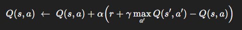
s, a: current state and action.r: reward.s′: next state.α: learning rate.
But we saw the problems:
Tables explode in high dimensions (Atari = millions of pixels).
Samples are correlated (consecutive frames).
Targets move with parameters, destabilizing learning.
Enter DQN: the solution that combines function approximation, replay, and target networks.
Step 2. The DQN Recipe
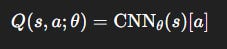
Architecture
Input: 4 stacked grayscale frames (84×84).
CNN extracts spatial-temporal features.
Fully connected layers output Q-values for all actions.
Training Objective
Sample minibatches from replay buffer D:
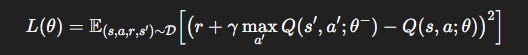
Online network with weights
θ.Target network with frozen weights
θ^-.Update
θ^-←θeveryCsteps.
Algorithm Outline
Initialize replay buffer
D.Initialize online net
Q(s, a; θ), target netQ(s, a; θ^−).For each step:
Select action (
ε-greedy).Execute, observe (
r, s′).Store transition in buffer.
Sample minibatch from buffer.
Compute targets with
θ^-.Update
θby gradient descent.Sync target network every
Csteps.
Visual:

Step 3. Worked Numerical Examples
Let’s bring this to life.
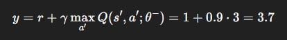
Example 1: Single Update with Target Network
Suppose transition:
State: paddle in middle.
Action: “move right.”
Reward:
r= 1.Discount:
γ= 0.9.Online
Qpredicts:Q(s, a)= 4.0.Target net predicts:
\max_{a’} Q(s’, a’)= 3.0.
Step 1: Compute target
Step 2: TD error
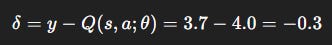
Step 3: Loss
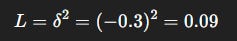
Interpretation: Online network was too optimistic (4.0). Update nudges prediction downward.
Visual:

Example 2: Replay Buffer Mini-Batch Update
Suppose minibatch = 2 samples:
Transition
A:
Q(s, a)= 2.0, reward = 0, next maxQ= 3.0.Target
y_A= 0 + 0.9 ⋅ 3 = 2.7 .Error
δ_A= 2.7-2.0 = 0.7.Loss_
A= 0.49.
2. Transition B:
Q(s, a)= 5.0, reward = 2, next maxQ= 4.0.Target
y_B= 2 + 0.9 ⋅ 4 = 5.6.Error
δ_B= 5.6–5.0 = 0.6.Loss_
B= 0.36.
Mini-batch loss:
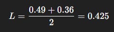
Interpretation: By sampling multiple experiences, replay buffer reduces variance and balances updates across diverse transitions.
Visual:

Step 4. Why DQN Changed Everything
DQN introduced three crucial stabilizers:
Replay Buffer: breaks correlations, improves efficiency.
Target Networks: stabilize moving targets.
CNN Function Approximators: handle raw pixels.
This cocktail turned Q-learning into a general-purpose deep RL algorithm.
Impact:
Learned 49 Atari games from scratch.
Sometimes beat human players.
Laid the foundation for Double DQN, Dueling DQN, Prioritized Replay.
Visual:

Special: Learn More in Learning to Learn: Reinforcement Learning Explained for Humans
In my book, I guide readers from tabular RL → DQN…
Get it here:
Closing
Classic Q-learning couldn’t handle high-dimensional spaces.
DQN = Q-learning + CNN + Replay Buffer + Target Networks.
We solved two worked examples:
Online prediction corrected downward (4.0 → 3.7 target).
Replay buffer minibatch average loss = 0.425.
DQN marked the true beginning of Deep RL.
Next: Double DQN: how to fix overestimation bias in Q-values.
Follow and Share
You can follow me on Medium to read more: https://medium.com/@satyamcser
#ReinforcementLearning #DeepRL #DQN #ExperienceReplay #TargetNetworks #CNN #TDLearning #Atari #MachineLearning #AIExplained #MLMath #satmis